Volatility Clustering and GARCH
Opening
In financial time series data, it is common to observe volatility clusturing, meanining large changes tend to be clustered. For example, the figure below shows daily returns (light blues) of the S&P500 index where one can observe clusters of larges changes during 2009 (financial crisis) and 2020 (Covid-19 stress).
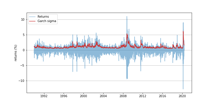
This post demonstrates how the volatility clustering phenomena can be analysed using Garch(1,1), one of the model simplest models featuring heteroskedasticity (a fancy word indicating that the volatility is varying over time as indicated by the red line in the above figure.)
Garch(1,1) Model
Following Section 21.2 of Hamilton’s Time Series Analysis (also wiki page as well), an $\mathrm{GARCH}(r,m)$ process for a standard deviation variable $h_t$ is described by
\[\begin{equation} h_t = \zeta + \frac{\alpha(L)}{1-\delta(L)} u_t^2 \nonumber \end{equation}\]where
- $L$ is the time lag operator (i.e. $L(x_t) = x_{t-1}$)
- $u_t := \sqrt{h_t} v_t$ with $v_t$ being an i.i.d. innovation with zero mean and unit variance
- $\alpha(\cdot)$ and $\delta(\cdot)$ are polynomials of order $m$ and $r$, respective, given as:
Taking $m=r=1$, GARCH(1,1) is written as
\[\begin{equation} h_t = (1-\delta_1) \zeta + \delta_1 h_{t-1} + \alpha_1 h_{t-1} v_{t-1}^2 \label{E:garchoo-hamilton} \end{equation}\]with the following restrictions:
- For $h_t \ge 0$, set $(1-\delta_1) \ge 0$, $\delta_1 \ge 0$ and $\alpha_1\ge 0$.
- For covariance-stationary $u_t^2$, set $\delta_1 + \alpha_1 < 1$.
Then, the unconditional mean $E[u_t^2]$ of $u_t^2$ is given by
\[\begin{equation} E[u_t^2] = \frac{(1-\delta_1)\zeta}{1-\delta_1-\alpha_1} \end{equation}\]Applying to Volatility of Stock Price
Suppose that the dynamics for return variable $r_t$ of stock price $S_t$ is given by
\[\begin{equation} r_t = \mu + \sigma_t \epsilon_t \label{E:garch-return} \end{equation}\]where
- $\epsilon_t$ is the innovation variable, assumed to be Gaussian (for simplicity) and i.i.d. over time.
- $\mu$ is the drift parameter for $r_t$.
- $\sigma_t$ is the volatility variable.
To model the dynamics of $\sigma_t$ using the GARCH(1,1) process (\ref{E:garchoo-hamilton}), make the following substitutions
\[\begin{equation} h_t \rightarrow \sigma_t^2,\quad \delta_1 \rightarrow \delta, \quad \alpha_1 \rightarrow \alpha, \quad E[u_t^2] \rightarrow \sigma_{\infty}^{2}, \quad v_t \rightarrow \epsilon_t \nonumber \end{equation}\]and obtain \(\begin{equation} \sigma_{t}^2 = \sigma_\infty^2(1 - \delta-\alpha)+ \delta \sigma_{t-1}^2+ \alpha \sigma_{t-1}^2 \epsilon_{t-1}^2 \label{E:garch-vol} \end{equation}\)
where $\sigma_\infty$, $\delta$ and $\alpha$ are constant model parameters with restrictions
\[\sigma_\infty > 0,\quad \delta \ge 0, \quad \alpha \ge 0,\quad \delta + \alpha < 1.\]Re-writing the equation above, it is easy to see that the Garch volatility $\sigma_t$ is mean-reverting: \begin{equation} \sigma_{t+1}^2 - \sigma_{t}^2 = (1 -\delta - \alpha)(\sigma_{\infty}^2 - \sigma_{t}^2) + \alpha\sigma_{t}^2 ( \epsilon_{t}^2 - 1 ) \end{equation} where $\sigma_\infty^2$ is the mean-reverting level, $(1-\delta-\alpha)$ is the mean-reverting speed, and $\alpha$ is the ‘vol of vol’.
Garch Filtering
Denoting the index price time series as
\[S_0, S_1, \cdots, S_t, \cdots,\]the goal is to derive the Garch volatility time series (red line in the above figure)
\[\sigma_0, \sigma_1, \cdots, \sigma_t, \cdots.\]To this end,
- Set $r_t$ is the log-change of $S_{t}$, i.e.
- $\mu$ and $\sigma_\infty$ are set to the unconditional mean and standard deviation of ${r_t}$ over all available data, respectively.
- For now, we set $\delta = 0.9$ and $\alpha = 0.09$, which would be within typical ranges (based on google search). The estimation method is discussed later this document.
Then, $\sigma_t$ can be derived using the following simple recursive algorithm:
- Initialise: \(\sigma^{2}_{0} = \sigma^{2}_{\infty}\) (or any other value as long as you can defend the choice)
- Assume that we have the volatility $\sigma_t$ as of time $t$. Then,
- Set the innovation term $\epsilon_t = (r_t - \mu) / \sigma_t$, which is from (\ref{E:garch-return}).
- Set the next volatility $\sigma_{t+1}$ using (\ref{E:garch-vol}).
The above algorithm produces the corresponding innovation time series (illustrated figure below)
\[\epsilon_1, \cdots, \epsilon_t, \cdots,\]which are daily returns with Garch volatilities removed.
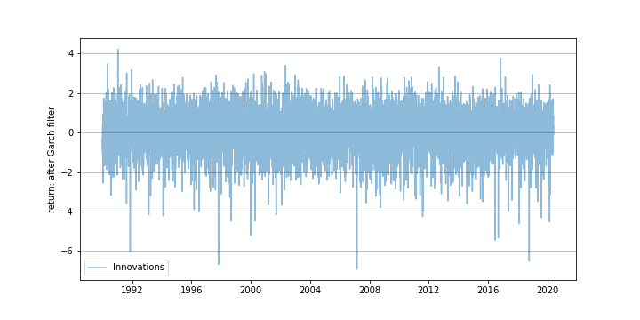
While one may run many statistical tests, it is visually obvious that the filtered returns ($\epsilon_t$) are more i.i.d. than the original returns ($r_t$). So, from the statistically perspective, the former samples are more meaningful to work with.
Simulation
To simulate a sample path using Garch(1,1), we generate samples for the innovation variable $\epsilon_t$. For illustration purposes, the standard normal random variable is used although other variables such as Student-t distributions can be used as well.
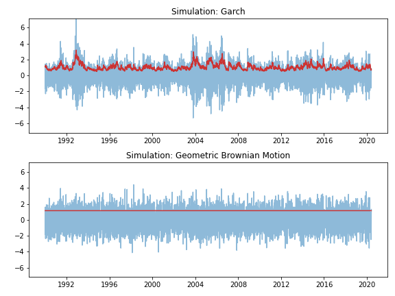
- The top/left figure below shows simulated returns (in light blue) using Garch(1,1) together with the corresponding Garch volatilities (in red). Volatility clustering pheonomena are clearly visible.
- In contrast, the bottom/left figure shows simulated returns when the geometric brownian motion (GBM) is applied (by setting $\delta=\alpha=0$) with constant volatility $\sigma_\infty$.
| returns | levels |
|---|---|
 |
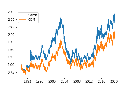 |
Finally, for simulated price paths, set an initial value, say 0, and sum the returns cumulatively, and take the exponential to obtain the paths in the right figure above.
Estimation: MLE
So far, we have postulated certain values for $\delta$ and $\alpha$ without justifications. In this section, we estimate them by applying the standard maximum likelihood estimation method.
Objective Function
To this end, noting that $\sigma_t$ is determined one time step in advance:
\[r_t | \mathcal F_{t-1} \sim \mathcal N (\mu, \sigma_{t}^2),\]the likelihood function for time step $t$ is given as \begin{equation} l(r_{t}|\mathcal F_{t-1}) = \displaystyle \frac{1}{\sqrt{2\pi \sigma_{t}^2}}\exp\left( - \frac{(r_{t} - \mu)^2 }{ 2 \sigma_{t}^2 } \right). \end{equation} Thus, we can write the objective function to maximize as below after doing the usual steps (multiply over samples, take log to turn into sum, ignore constant factors) \begin{equation} L(\delta, \alpha) = -\sum_{t} \left[ \ln \sigma_{t}^2 + \frac{(r_{t} - \mu)^2}{ \sigma_{t}^2 }\right]. \end{equation}
Optimisation
Before running the actual optimisation function, we calculate $L$ over a range of $\delta$ and $\alpha$ values with constraint $\delta + \alpha < 1$ and obtain the following contour plot which indicates where the maximum is roughly located.
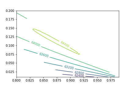
Running an optimisation routine (e.g. Nelder-Mead), the maximum is achieved at
\[(\delta, \alpha) = (0.88035162, 0.10633708),\]which is not too far from our postulated values (0.9, 0.09).
vs EWMA
When $\delta+\alpha=1$, we have
\[\sigma_{t+1}^2 = \delta \sigma_{t}^2 + (1-\delta) \left( r_t - \mu \right)^2\]which can be easily shown to be the EWMA volatility.