Kalman Filter
This post is about how the Kalman Filter works based on Chapter 13 of Time Series Analysis by Hamilton.
- The Wikipedia page is also pretty good.
- Youtube on Bayesian/Kalman
Note on Kalman Gain $K_t$:
- In Hamilton, it is defined as $K_t := FP_{t\vert t-1}H(H’P_{t\vert t-1}H+R)^{-1}$.
- In other literature (including the wikipedia), it is defined as $K_t := P_{t\vert t-1}H(H’P_{t\vert t-1}H + R)^{-1}$
In this post, we follow the Hamilton’s notation.
Illustration of 1D
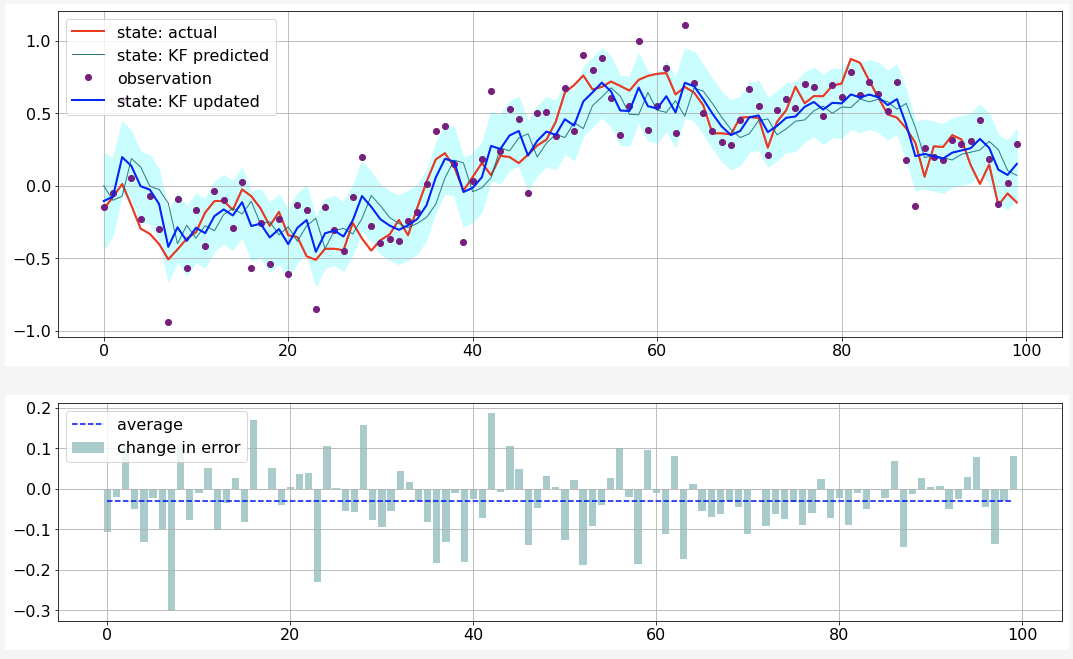
- parameters: $F = 0.95$, $A=1$, $H=1$, $Q=0.1^2$, $R=0.2^2$
- top plot
- red: actual state variable
- blue (dashed): predicted state variable
- blue (solid): updated state variable
- bottom plot:
- bars: changes in errors before and after Kalman update |updated - actual| - |predicted - actual|
- dashed line: average changes.
- code here
Setup
Notation:
- $p(x)$: pdf of a random vector
- $f(x; \mu, \Sigma)$: pdf of multivariate normal distribution
State-Space Representation
The Kalman Filter is used to infer the hidden process $\vec X_t$ (known as state variable) from an observed process $\vec Y_t$. The setup is the state-space represenation of $\vec Y$:
\[\begin{eqnarray} \color{red} \vec X_{t} & = & \color{red} F X_{t-1} + \vec v_{t} \label{E:state-eq} \\ \color{green} \vec Y_{t} & = & \color{green} A' \vec U_{t} + H' \vec X_{t} + \vec w_{t} \label{E:obs-eq} \end{eqnarray}\]where $F$, $A$ and $H$ are matrics, $\vec v_t$ and $\vec w_t$ are white noises with \begin{equation} E(\vec v_t \vec v_\tau’) = \mathbf{1}_{t = \tau} \cdot Q, \quad E(\vec w_t \vec w _\tau’ ) = \mathbf{1} _{t = \tau} \cdot R, \quad \textrm{and} \quad E(\vec v_t, \vec w _\tau) = 0, \end{equation} and $\vec U_t$ is exogenous (predetermined at $t-1$, for example, lagged values of $\vec Y$ or variables uncorrelated with $\vec X$.)
We drop $\ \vec{}\ $ to simplify the notation unless absolutely required.
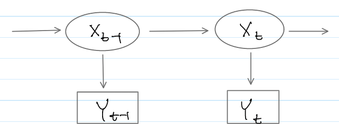
Another View: Hidden Markov Model
Resembling a hidden Markov model (HMM) (see the diagram below), the state-space representation provides the following conditional probabilities
- $\color{red} p(X_{t}\vert X_{t-1})$ from state equation (\ref{E:state-eq})
- $\color{green} p(Y_{t}\vert X_{t}, U_{t})$ from observation equation (\ref{E:obs-eq})
Roughly speaking, the task is to find the probability distribution for $X_t$ given exogenous variable $u_s$ and observation $y_s$: \begin{equation} \color{blue} p(X_{t} | y_t, y_{t-1}, \cdots, y_1, u_t, u_{t-1}, \cdots, u_1). \end{equation}
Kalman Filtering
Let $\mathcal F_t$ be the set of data observed through time $t$ \begin{equation} \mathcal F_t := y_{1:t} \cup u_{1:t} = \{ y_t, y_{t-1}, \cdots, y_{1}, u_t, u_{t-1}, \cdots, u_{1} \} \end{equation} where $y_s$ and $u_s$ are the observations for $Y_s$ and $U_s$, respectively.
Recursive Process
The filter produces three sets of random vector time series over time $t$.
| step | time | random vector | mean | covariance |
|---|---|---|---|---|
| forecast $X_t$ (a priori) | $t-1$ | $\color{teal} X_{t \vert t-1} := X_t \vert \mathcal F_{t-1}$ | $\color{teal} \hat{x}_{t \vert t-1}$ | $\color{teal} P_{t \vert t-1}$ |
| forecast (predicted) $Y_t$ with exogenous variable $u_t$ | $t-1$ | $\color{orange} Y_{t \vert t-1} := Y_t \vert { u_t, \mathcal F_{t-1} }$ | $\color{orange} \hat{y}_{t \vert t-1}$ | $\color{orange} S_{t \vert t-1}$ |
| update $X_t$ (a posteriori) with new observation $\color{purple} y_t$ | $t$ | $\color{blue} X_{t \vert t} := X_t \vert { \mathcal F_{t} } = X_t \vert { {\color{purple} y_t}, u_t, \mathcal F_{t-1} }$ | $\color{blue} \hat{x}_{t \vert t}$ | $\color{blue} P_{t \vert t}$ |
A few observations:
- Since $U_t$ is predetermined at $t-1$, it contains no information about $X_t$, thus \begin{equation} \color{teal} X_t \vert \mathcal F_{t-1} = X_t \vert \mathcal u_t, F_{t-1} \end{equation}
- As soon as the initial forecast $X_{1 \vert 0}$ is specified, the filtering starts to operate recursively.
- Since the state-space equations are linear and the innovations are white noise, all of these random vectors are Gaussians and thus fully described once their mean vectors and variance matrices are specified.
Algorithm
We (kind of) follows Hamilton’s Time Series Analysis….
The algorithm produces the following sequence \begin{equation} \underline{X_{1|0}} \to Y_{1|0} \to X_{1|1} \to X_{2|1} \to \cdots \to \underline{Y_{t|t-1}} \to \underline{X_{t|t}} \to \underline{X_{t+1|t}} \to Y_{t+1|t} \to \cdots \end{equation} and it is sufficient to describe how to obtain the underlined variables.
$X_{1|0}$: Initialisation
In the absence of any observations, set $\color{teal} X_{1\vert 0}$ to the unconditional distribution of $X_{t}$ (assuming covariance-stationary):
$Y_{t|t-1}$: Forecasting $Y_t$
The exogenous variable $u_t$ is assumed to predetermined at $t-1$.
From the observation equation (\ref{E:obs-eq}), marginalise to $X_t$ \(\begin{eqnarray} p({\color{orange} Y_{t|t-1}} = y) & := & p({\color{orange} Y_t = y | u_t, \mathcal F_{t-1}}) \nonumber\\ & = & \int_{x \in X_t} p({\color{green} Y_t} = y | {\color{green} X_t } = x, {\color{green} u_t, \mathcal F_{t-1}}) p({\color{teal} X_t = x | u_t, \mathcal F_{t-1}}) dx \nonumber\\ & = & \int_{x \in X_t} f(y; A'u_t + H x, R) f(x; {\color{teal} \hat x_{t|t-1}, P_{t|t-1}}) dx \label{E:y-pred-conv} \\ & := & f(y; {\color{orange} \hat y_{t|t-1}, S_{t|t-1}}). \nonumber \end{eqnarray}\) where (\ref{E:y-pred-conv}) is a Gaussian as a convolution of two Gaussians and the last equation is by definition.
While $\hat y_{t \vert t-1}$ and $S_{t\vert t-1}$ can be obtained by performing the convolution, it can be calculated directly using linear projections (to add a line):
- For $\color{orange} \hat y_{t\vert t-1}$: \(\begin{eqnarray} \color{orange} \hat y_{t|t-1} &:=& \hat E[{\color{orange} Y_t|u_t, \mathcal F_{t-1}}] \label{E:y-pred-mean-tower-a} \\ &=& \hat E[ E[{\color{green} Y_t | X_t, u_t, \mathcal F_{t-1}}]| u_t, \mathcal F_{t-1}] \label{E:y-pred-mean-tower-b}\\ &=& \hat E[ A'u_t + H' \color{teal} X_t | u_t, \mathcal F_{t-1} ] \nonumber \\ &=& A'u_t + H' \color{teal} \hat x_{t|t-1} \nonumber, \end{eqnarray}\) where a tower rule is applied to (\ref{E:y-pred-mean-tower-a}) to get (\ref{E:y-pred-mean-tower-b}).
- To derive $\color{orange} S_{t\vert t-1}$, the residual of $Y_t$ is given by \begin{equation} {\color{orange} Y_t - \hat y_{t\vert t-1}} = H’({\color{teal} X_t - \hat x_{t\vert t-1}}) + w_t \nonumber \end{equation} and thus \begin{equation} {\color{orange} S_{t\vert t-1}} := E[({\color{orange} Y_t - \hat y_{t\vert t-1} })({\color{orange} Y_t - \hat y_{t\vert t-1}})’] = H’{\color{teal} P_{t\vert t-1}}H + R. \nonumber \end{equation}
$X_{t|t}$: Updating the Inference about $X_t$
Taking into account the new observation $\color{purple} y_t$, the inference $\color{blue} X_{t\vert t}$ about $X_t$ is updated from the forecast distribution $\color{teal} X_{t\vert t-1}$
\[\begin{eqnarray} p({\color{blue} X_{t|t}} = x) & := & p({\color{blue} X_t}=x|{\color{blue} Y_t} = {\color{purple} y_t}, {\color{blue} u_t, \mathcal F_{t-1}}) \nonumber \\ & \propto & p( {\color{green} Y_t} = {\color{purple}y_t}|{\color{green} X_t}=x,{\color{green} u_t, \mathcal F_{t-1}}) p({\color{teal} X_t=x|u_t, \mathcal F_{t-1}}) \nonumber \\ & = & f({\color{purple} y_t}; A'u_t + H'x, R) f(x; {\color{teal} \hat x_{t|t-1}, P_{t|t-1}}) \nonumber \\ & := & f(x; {\color{blue} \hat x_{t|t}, P_{t|t}}) \nonumber \end{eqnarray}\]where the last equation is by definition.
Again, use the linear projection toolkits (TODO: add a link) to calculate $\hat x_{t\vert t}$ and $P_{t\vert t}$:
\[\begin{eqnarray} {\color{blue} \hat x_{t|t}} & := & \hat E(X_t|Y_t = {\color{purple} y_t}, u_t, \mathcal F_{t-1}) \nonumber \\ & = & \hat E({\color{teal} X_t | u_t, \mathcal F_{t-1}}) + G_{XY}G_{YY}^{-1} ({\color{purple} y_t} - {\color{orange} \hat E(Y_t|u_t, \mathcal F_{t-1})}) \nonumber \\ & = & {\color{teal} \hat x_{t|t-1}} + G_{XY}{\color{orange} S_{t|t-1}}^{-1} ({\color{purple} y_t} - {\color{orange} \hat y_{t|t-1}}) \nonumber \\ & = & {\color{teal} \hat x_{t|t-1}} + {\color{teal} P_{t|t-1}}H(H' {\color{teal} P_{t|t-1}} H + R)^{-1} ({\color{purple} y_t} - A'u_t - H' {\color{teal} \hat x_{t|t-1}}) \nonumber \end{eqnarray}\]and
\[\begin{eqnarray} {\color{blue} P_{t|t}} & := & G_{XX} - G_{XY} G_{YY}^{-1} G_{YX} \nonumber \\ & = & {\color{teal} P_{t|t-1}} - {\color{teal} P_{t|t-1}} H(H' {\color{teal} P_{t|t-1}} H + R)^{-1} H' {\color{teal} P_{t|t-1}} \nonumber \end{eqnarray}\]where we have used
\[\begin{eqnarray} G_{YY} & := & E[(Y_t - \hat E(Y_t|u_t, \mathcal F_{t-1}))(Y_t - \hat E(Y_t|u_t, \mathcal F_{t-1}))'] = {\color{orange} S_{t|t-1}} \nonumber \\ G_{XY} & := & E[(X_t - \hat E(X_t|u_t, \mathcal F_{t-1}))(Y_t - \hat E(Y_t|u_t, \mathcal F_{t-1}))'] \nonumber \\ & = & E[(X_t - \hat x_{t|t-1})(H'(X_t - \hat x_{t|t-1}))'] = {\color{teal} P_{t|t-1}}H \nonumber \\ G_{XX}& := & E[(X_t - \hat E(X_t|u_t, \mathcal F_{t-1}))(X_t - \hat E(X_t|u_t, \mathcal F_{t-1}))'] = {\color{teal} P_{t|t-1}} \nonumber \end{eqnarray}\]
$X_{t+1|t}$: Forecasting $X_{t+1}$
This step is straightforward
\[\begin{eqnarray} {\color{teal} \hat x_{x+1|x}} & := & \hat E({\color{red} X_{t+1}|\mathcal F_{t}}) \nonumber \\ & = & \hat E( F X_t + v_{t+1} | \mathcal F_{t}) \nonumber \\ & = & F {\color{blue} \hat x_{t|t}} \nonumber \end{eqnarray}\]and
\[\begin{eqnarray} {\color{teal} \hat P_{t+1|t}} & := & E[({\color{teal} X_{t+1}-\hat x_{t+1|t}})({\color{teal} X_{t+1}-\hat x_{t+1|t}})'] \nonumber \\ & = & E[({\color{red} F X_t + v_{t+1}} - F {\color{blue} \hat x_{t|t}})({\color{red} F X_t + v_{t+1}} - F {\color{blue} \hat x_{t|t}})'] \nonumber \\ & = & F {\color{blue} P_{t|t}} F' + Q \nonumber \end{eqnarray}\]
Maximum Likelihood Estimation of Parameters
The forecast algorithm for $Y_t$ provides the likelihood of observation $y_t$ \begin{equation} p({\color{orange} Y_t=y_t|u_t, \mathcal F_{t-1}}) = f(y_t; A’u_t + H’ \hat x_{t|t-1}, H’P_{t|t-1}H +R), \end{equation} allowing us to set up a log-likelihood function \begin{equation} \sum_{t=1}^{T} \log f(y_t; A’u_t + H’ \hat x_{t|t-1}, H’P_{t|t-1}H +R), \end{equation} which is maximised with respect to $F$, $Q$, $A$, $H$ and $R$.
Application to Term Structure Models
Following Section 7 of Duffee & Stanton….
Model
The short rate $r_t$ is given by \begin{equation} r_t = \varphi + x_{1t} + \cdots + x_{nt} \end{equation} where each factor $x_{it}$ has a mean-reverting dynamics in the risk neutral measure $\mathcal Q$.
\begin{equation} dx_{it} = -k_i x_{it} dt + \sigma_i dW^{\mathcal Q}_{it} \label{E:mr-eq-q} \end{equation} where $W^{\mathcal Q} _{it}$ is a Brownian process under $\mathcal Q$. This is a generalisation of the G2++ model in Brigo & Mecurio.
Being an affine term-structure model, one can write the price $P_t(\tau)$ of a zero-coupon bond with maturity $\tau$:
\[\begin{eqnarray} P_t(\tau) & = & E^{\mathcal Q} \left[ \exp\left(-\int_{t}^{t+\tau} r_s ds \right) \right] \nonumber \\ & = & \exp\left( - \varphi \tau + \sum_{i} \alpha_{i}(\tau) + \sum_{i} \beta_{i}(\tau) x_{it} + \mathcal V_t(\tau) \right) \label{E:bond-price} \end{eqnarray}\]Here, $\alpha_{i}(\tau)$ and $\beta_{i}(\tau)$ are simple functions with parameters only appearing in (\ref{E:mr-eq-q}) whereas $V_t(\tau)$ have a more complex form, mixing parameters across (\ref{E:mr-eq-q}) and correlations among $W_{it}$. Thus, for simplicity, the Brownian motions are assumed to independent to have $\mathcal V_t(\tau) = 0$. With this assumption, the yield rate $y_t(\tau)$ is defined as \begin{equation} e^{-\tau y_t(\tau)} = P_t(\tau)\quad\textrm{or}\quad y_t(\tau) = \varphi - \sum_{i} \frac{\alpha_{i}(\tau)}{\tau} - \sum_{i} \frac{\beta_{i}(\tau)}{\tau} x_{it}. \label{E:yield-formula} \end{equation} which is linear in $x$.
State-Space Equations
State Equation: For the state equation for the factors $x_t$, the first step is to introduce the price of risk to the dynamic model (\ref{E:mr-eq-q}) under $\mathcal Q$ to obtain the model under the real (physical) measure $\mathcal P$. For example, we assume \begin{equation} dx_{it} = (\lambda_i-k_i x_{it}) dt + \sigma_i dW_{it} \quad \textrm{under} \quad \mathcal P \label{E:mr-eq-p} \end{equation} where $\lambda_i$ is a constant price of risk term. Then, the state equation is given as \begin{equation} X_{t+1} = G + F X_{t} + v_{t+1} \end{equation} where $G_i = \lambda_i$ and $F_{ij} = \delta_{i,j}(1 - k_i)$ and $E[v_{it}v_{jt}] = \delta_{i,j} \sigma_{i}^2$.
Observation Equation: Defining the observation vector as the term-structure of the yield rates over a set of maturities $\tau_{1}$, $\cdots$, $\tau_{n}$, the observation equation is based on (\ref{E:yield-formula}): \begin{eqnarray} Y_{t} = A’U_{t} + H’X_{t} + w_t \end{eqnarray} where $A_{ij} = \varphi - \frac{\alpha_i(\tau_j)}{\tau_j}$, $U_{it}=1$ and $H_{ij} = -\frac{\beta_{i}(\tau_j)}{\tau_j}$ where $i=1, \cdots, n$ and $j=1, \cdots, m$.
Filtering
The application of the Kalman filter goes like this:
- From time series of $y_{t}$, estimate the model parameters.
- Infer the factors $x_{t\vert t}$
- Simulate $x_{t}$ using the state equation for $t$ in future.
- Construct the yield curve at $t$ using \ref(E:yield-formula).