Parameter Estimation of Ornstein-Uhlenbeck Process
Ornstein-Uhlenbeck Process
The Ornstein-Uhlenbeck (OU) process is one of the simplest mean-reverting process with many applications including modelling financial time series such as interest rates (known as the Vasicek model in such a context).
Mathematically, the process $X_t$ is defined as \begin{equation} dX_t = -\theta ( \mu - X_t) dt + \sigma dW_t \nonumber \end{equation} where $W_t$ is a Brownian motion, $\mu$ is the long-term level, $\theta > 0$ is the mean-reversion speed and $\sigma$ is the volatility of the process. Discretizing in time with $\delta = 1$, the equation is written as a standard AR(1) process \begin{equation} X_t = \alpha + \beta X_{t-1} + \sigma \epsilon_t \nonumber \end{equation} with \begin{equation} \theta = 1-\beta,\ \mu=\alpha/\theta, \nonumber \end{equation} where $\epsilon_t \sim N(0,1)$ and i.i.d. across $t$.
Textbook Approach - Potentially Unstable
Given time series data $x_1, \cdots, x_t$, a standard textbook approach for estimating this process is to apply the maximum likelihood estimiation (MLE) to innovations $\epsilon_t$ (e.g. Chap 5, Time Series Analysis by Hamilton), which turns out to be equivalent to the OLS regression \begin{equation} y_{t} = \alpha + \beta x_{t} + \eta_t \end{equation} where $y_t := x_{t+1}$ and $\eta_t := \sigma \epsilon_{t+1}$
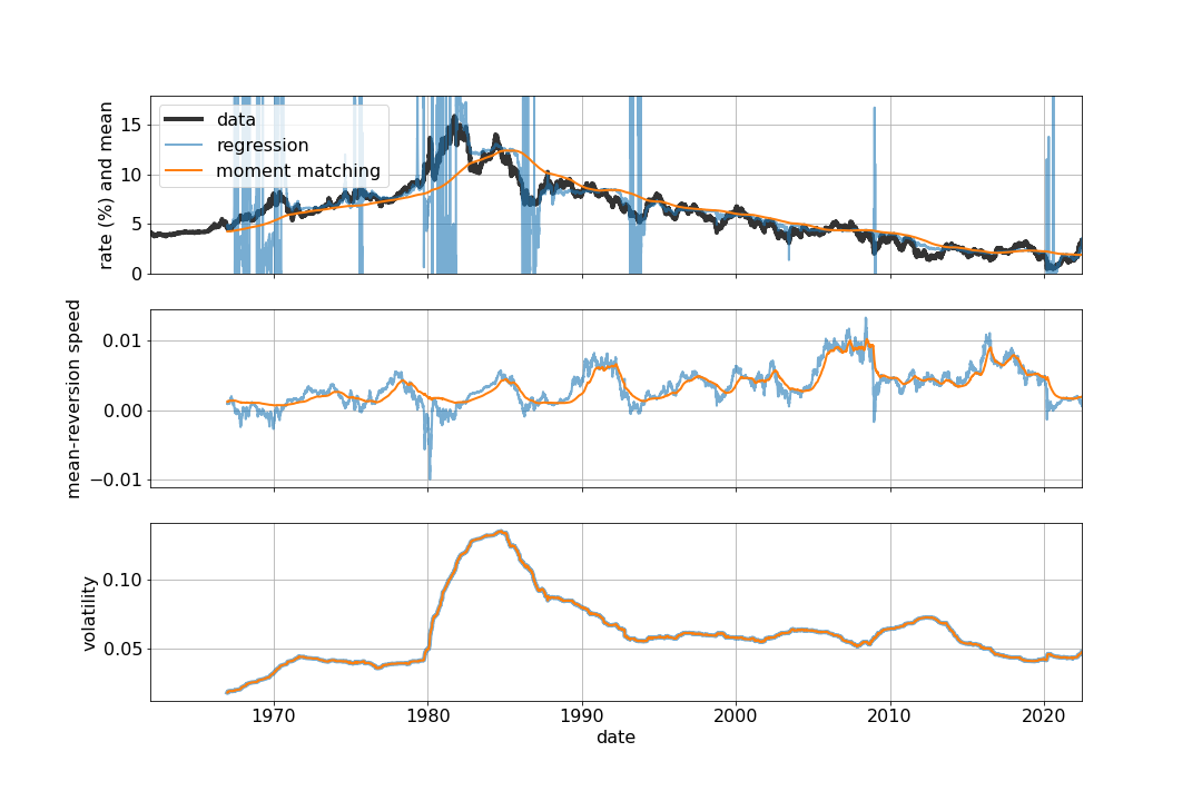
We apply this method to time-series data of 10y US treasury yields (data source) and estimate the OU parameters for each rolling-window with 1250 data points (about 5 years). The resulting parameters are illustrated in blue in the figure below.
- top: mean $\mu$ (blue and orange) and underlying data (black)
- middle: mean-resersion speed $\theta$
- bottom: volatility $\sigma$. The two lines are almost on top of each other. In each plot, the blue and orange lines are obtained from the regression and momentum matching methods, respectively.
Unfortunately, this method is unstable as it can (and does in this example) produce negative mean-reversion rate $\theta$, making the process mean-diverting! For example, from the middle figure, negative estimated values of $\theta$ are observed in early 2020 (Covid), 2008 (Financial Crisis), and most previous crisis periods. When $\theta$ becomes negative, the estimated means $\mu$ start fluctuated unstably (top figure), making the model unusable.
Momentum Matching - Stable Alternative
A stable estimation method can be obtained by matching three moments:
- long term mean: $E[X_t] = \mu$
- (unconditional) variace: $\mathrm{Var}[X_t] = \sigma^2/(1-\beta^2)$
- variace of increment: $\mathrm{Var}[X_t - X_{t-1}] = (1-\beta)^2 \mathrm{Var}[X_t] + \sigma^2$ where one can show
The only remaining task is to specify appropriate estimators for given time series observation $x_1, \cdots, x_n$.
For illustration purposes, we consider the following estimators:
| $E[X_t]$ | $\mathrm{Var}[X_t]$ | $\mathrm{Var}[X_t-X_{t-1}]$ |
|---|---|---|
| sample average of $x_{t}$ | sample variance of $x_{t}$ | sample variance of $x_{t}-x_{t-1}$ |
The estimated parameters are shown in the figure above using orange lines. Observe
- The estimated processes are always mean-reverting as $\theta$ is positive.
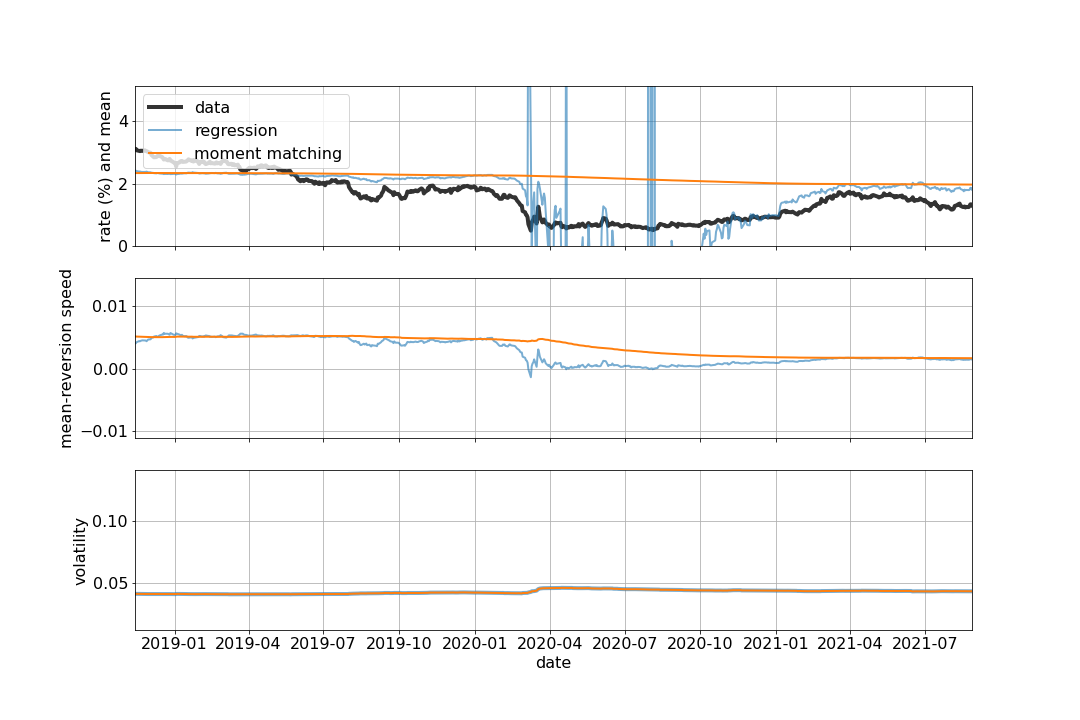
- Broadly speaking, both methods produce comparable parameters as long as the regression method produces reasonably positive $\theta$. For example, see the zoom-in figure below:
In closing, it is worth having a few notes:
- Different estimators can be used (e.g. $E[X_t]$ could be estimated using the medien).
- Having stable and less volatile parameters does not mean that the model has a better forecasting capability. The model should be backtested.
- For codes use to create plots, here