Numba and Numpy

Jupyter notebook

Background

Personally, numpy is the most important package because of its vectorisation implementation. Generally speaking, it makes the code shorter, easier to read, and most importantly faster, in fact, much faster if compared to nativa Python. But, the catch is generally. Certain algorithms or procedures are not natually vectorisable and the resulting vectorised codes can have awkward structures that are difficult to read. They may also introduce uncessary but unavoidable overheads. This problem can be solved using numba, which compiles python codes behind-the-scene into fast machine codes.

Illustration - MC with MC

Recently, I had to implement to simulate a Markov chain model, requiring a large number of Monte Carlo scenarios (order of 10M). We started using numpy and it was fast. But, we wanted faster, and realised that the model is a good example where the vectorisation approach adds unnessary overheads that are unavoidable with numpy. So, we considered numba.

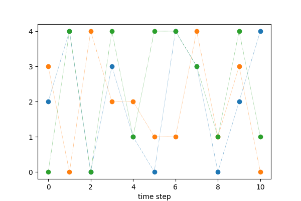
Markov Chain

Source: Wikipedia

A (discrete-time) markov chain is a stochastic model with many real life applications. See the relevant Wikipedia page for more information. The model is described in terms of

• a finite set of states
• transition probabilities from one state to another state

To simulate a markov chain,

• set the intial state
• draw a uniform random number between 0 and 1
• compare to the cumulative transition probabilities to determine the next state
• repeat

Implementation

For benchmark purposes, three functions are implemented to simulate the model:

1. Native Python
2. Native Python with numby (via njit)
3. Numpy implementation

Here is a code block. Only the first function is documented. The other two functions have the same arguments and return values.

# Nativa Python version
def markov_chain_simulation_naive(v_curr_state, v_draw, mtx_CTP0):
    """Markov chain simulation

    Args:
        v_curr_state (1-d numpy vector, integer): vector of current states
        v_draw (1-d numpy vector, float): vector of uniform random numbers between 0 and 1
        mtx_CTP0 (1-d numpy matrix, float): cumulative transition probability matrix without the last column (which consists of ones by definition)

    Returns:
        1-d numpy vector, integer: vector of next states
    """

    v_next_state = np.empty_like(v_curr_state)
    for n in range(v_next_state.size):
        curr_s = v_curr_state[n]
        v_next_state[n] = digitize_scalar_nb(v_draw[n], mtx_CTP0[curr_s])
    
    return v_next_state


# Nativa Python version (identical to above), numba'ed
@njit(fastmath=True, cache=True)
def markov_chain_simulation_nb(v_curr_state, v_draw, mtx_CTP0):
    v_next_state = np.empty_like(v_curr_state)
    for n in range(v_next_state.size):
        curr_s = v_curr_state[n]
        v_next_state[n] = digitize_scalar_nb(v_draw[n], mtx_CTP0[curr_s])
    return v_next_state

# Numpy implementation
def markov_chain_simulation_np(v_curr_state, v_draw, mtx_CTP0):
    v_next_state = np.empty_like(v_curr_state)
    for s in range(0, mtx_CTP0.shape[0]):
        mask = v_curr_state == s
        v_next_state[mask] = np.digitize(v_draw[mask], mtx_CTP0[s])
    return v_next_state

Observe that the native Python code, which is numba’ed, is as simple as the numpy version. In fact, I argue that it is simpler and easier to understand.

Simulations

First, the number of states should be specified together with the transition probabilities among them. The cumulative probabilities are required as inputs to the simulation

# number of states
num_state = 5

# define transition probability matrix
mtx_TP = np.random.uniform(0.0, 1.0, (num_state, num_state))
mtx_TP /= np.sum(mtx_TP, axis=1, keepdims=True)

# cumulative transition probability matrix
mtx_CPT = np.cumsum(mtx_TP, axis=1)

Then, we simulate the model over several steps for a large number of scenarios.

num_step = 10
seed = 1234

num_draw = 1000000

# initialise
v_init_state = np.random.randint(0, num_state, num_draw)

# simulation: naive
rng = np.random.default_rng(seed)
td = 0.0
v_next_naive = v_init_state.copy()
for n in range(num_step):
    v_draw = rng.uniform(0.0, 1.0, num_draw)
    t0 = time.time()
    v_next_naive = markov_chain_simulation_naive(v_next_naive, v_draw, mtx_CPT0)
    td += time.time() - t0
print('naive: ' + str(td) + ' seconds')

# ..... omitted for numba and numpy simulations ......

Results

• When 1M scenarios over 10 steps are used: The numba verison (0.12 seconds) is
  • over 50 time faster than the naive version (6.7 seconds)
  • over 3 time faster than the numpy version (0.43 seconds)
• When 10M scenarios are used, the numba version (1.39 seconds) is again over 3 times fater than the numpy version (4.98 seconds).

In Closing

In this post, we have provided an illustrative example where numba can be used to speed up Markov chain simulations. Not only the numba’ed native Python code is actually simpler than the numpy version, it is noticeably faster; in our experiments, over 3 times faster.

So, numba is a great supplementary package that can be utilised when procedures/algorithms are not easily vectorisable.