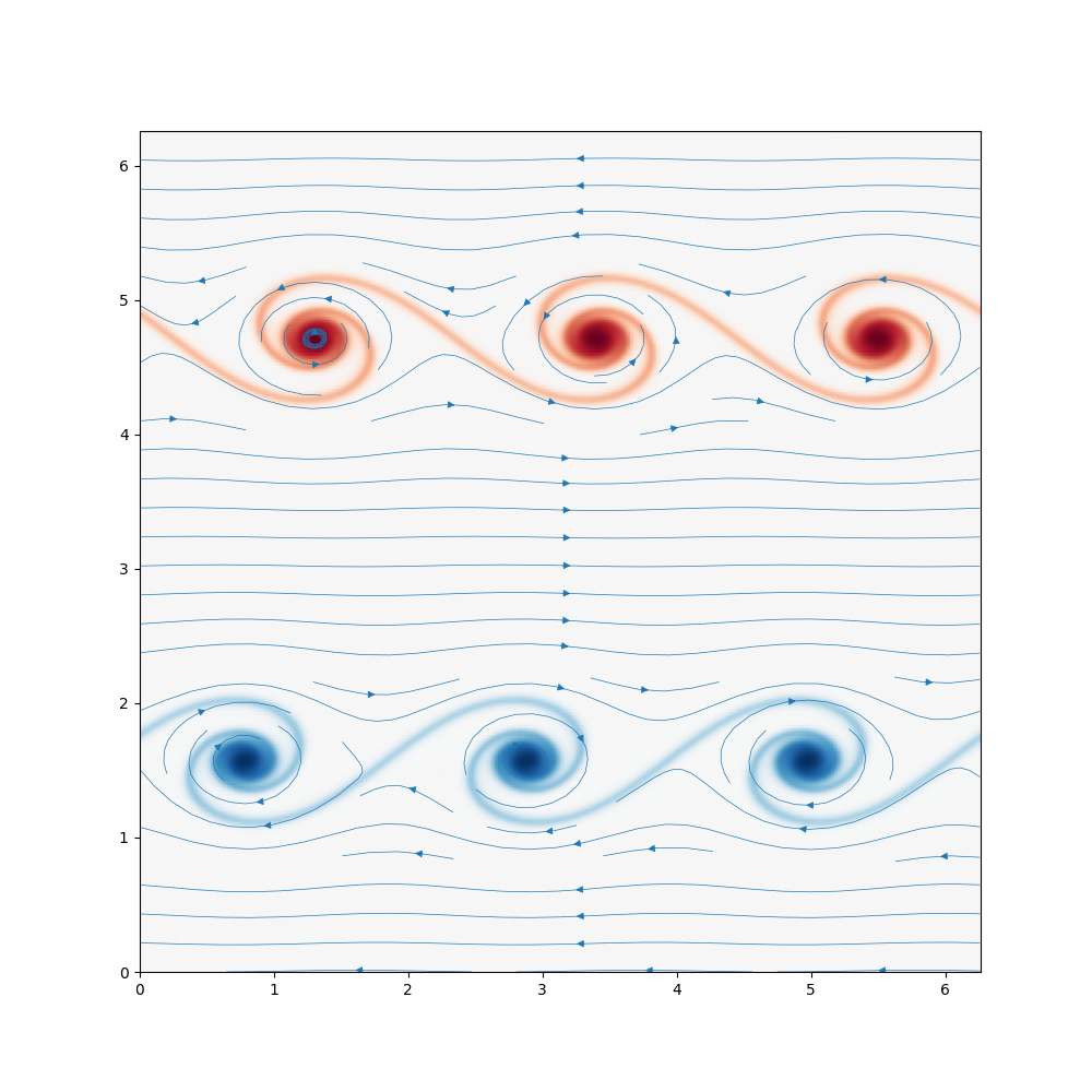
Kelvin Helmholtz	2D Turbulence

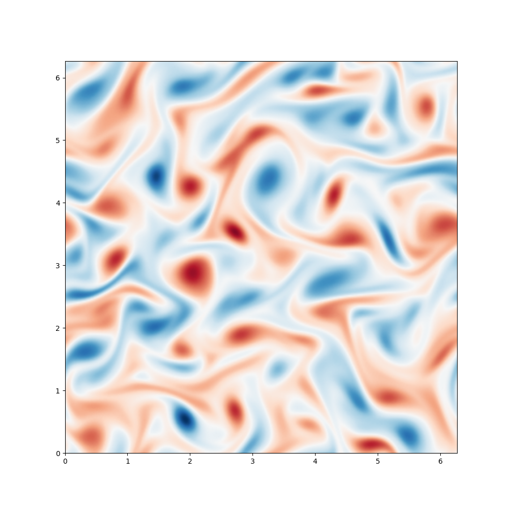This post is about simulating the 2D incompressible Navier Stokes equations in a rectangular domain with the period boundary conditions in both axes. This was a topic I studied in my graduate school days when I used C/C++ and Fortran to implement the core model and Matlab for plotting purposes. The purpose of this post is just for me to remind of those equations and techniques back for no particular reason.

Equations

The 3D incompressible Navier-Stokes equations (wiki) are given by

\[\begin{eqnarray*} \frac{D}{Dt}\vec{u} + \vec\nabla p & = & \nu \nabla^2 \vec{u} \\ \vec{\nabla}\cdot \vec{u} & = & 0. \end{eqnarray*}\]

where $\vec{u} = [u,v,w]$ is the velocity vector field, $p$ is the pressure field, and $\frac{D}{Dt}$ is the material derivative, defined as $\frac{D}{Dt} = \frac{\partial}{\partial t} + \vec{u}\cdot \vec{\nabla}.$

If restricted to the 2D case where $w = 0$, we can introduce a stream function $\psi$ such that \begin{equation} u = \frac{\partial \psi}{\partial y} \quad\textrm{and}\quad v = -\frac{\partial \psi}{\partial x} \label{E:def-stream-func} \end{equation} so that the divergence-free condition $\nabla\cdot \vec{u} = 0$ is satisfied. Taking the curl $\vec{\nabla} \times$ of the first NS equation, the third component becomes \begin{equation} \frac{\partial}{\partial t} \nabla^2 \psi + \frac{\partial \psi}{\partial y} \frac{\partial}{\partial x} \nabla^2 \psi - \frac{\partial \psi}{\partial x} \frac{\partial}{\partial y} \nabla^2 \psi = \nu \nabla^2 \nabla^2\psi \end{equation} In terms of vorticity $\omega = - \nabla^2 \psi$, \begin{equation} \frac{\partial \omega}{\partial t} + \frac{\partial \psi}{\partial y} \frac{\partial \omega}{\partial x} - \frac{\partial \psi}{\partial x} \frac{\partial \omega}{\partial y} = \nu \nabla^2 \omega. \label{E:ns2d-omega} \end{equation}

Numerical Simulation using Spectral Method

If the periodic boundary condition is assumed, it is straightforward to implement the 2D equation using the standard spectral method with a standard ODE solver such as Runge-Kutta methods.

Fourier Transform

To this end, take the (discrete) Fourier transform $\mathcal F$ of (\ref{E:ns2d-omega}) \begin{equation} \frac{\partial \hat\omega}{\partial t}(\vec{k}) + \mathcal F \left[J\right] (\vec{k}) = - \nu k^2 \hat\omega(\vec{k}). \label{E:ns2d-omega-k} \end{equation} where $\hat{\omega}(\vec{k})$ is the Fourier coefficient at the Fourier model $\vec{k}$ and $J$ is the nonlinear term (known as Jacobian) $J = \frac{\partial \psi}{\partial y} \frac{\partial \omega}{\partial x} - \frac{\partial \psi}{\partial x} \frac{\partial \omega}{\partial y}.$ and $\mathcal F \left[J\right]$ is its Fourier transform.

Time integration

While one may apply an ODE solver directly to (\ref{E:ns2d-omega-k}), we can first integrate the diffusion term analytically for each time step. \begin{equation} \frac{\partial e^{\nu k^2 t} \hat\omega}{\partial t}(\vec{k}) + e^{\nu k^2 t} \mathcal F \left[J\right] (\vec{k}) = 0 \label{E:ns2d-omega-k-int} \end{equation}

We apply the standrad RK4 method (wiki) to the above system of equations over $\vec{k}$’s. For stabilty of the scheme, the time step $\delta t$ is set to be small enough so that an appropriate CFL condition is met (see wiki). In particular, we consider the following CFL value based on the Jacobian term in (\ref{E:ns2d-omega}) \begin{equation} C = \delta t \left[ \frac{\max |u|}{\delta x} + \frac{\max |v|}{\delta y}\right] \end{equation} and ensure it to be within the RK4 stability region, or $C < C_{\max} \approx 2.8.$ Note that the diffusion term is not considered in specifying $C$ as it is analytically integrated in (\ref{E:ns2d-omega-k-int}).

Discrete Fourier Transform

A python wrapper pyfftw to a very popular FFT liborary FFTW is used to compute any discrete Fourier transformations. See also my own post on fftw. For a 1D array, for example, the wrapper provides (i) the forward “physical to Fourier” transform \begin{equation} Y_k = \sum_{j=0}^{n-1} X_j e^{-2\pi i k j / n}, \end{equation} and (ii) the backward “Fourier to phyiscal” transform \begin{equation} X_j = \frac{1}{n}\sum_{k=0}^{n-1} Y_k e^{2\pi i k j / n}. \end{equation}

Fourier decomposition

For a function $u(x)$ periodic in $[0, L]$, its Fourier decomposition is written as \begin{equation} u(x) = \frac{1}{n} \sum_{k=0}^{n-1} \hat u_k e^{i \left( 2\pi k / L \right) x } = \frac{1}{n} \sum_{k=-n/2+1}^{n/2} \hat u_k e^{i \left( 2\pi k / L \right) x }, \end{equation} where the $k$-th wave-length is $2\pi k /L$.

Calculation of Jacobian and Dealiasing

To calculate the Fourier transform of the products appearing in the Jacobian term, we use the standard procedure:

apply the `3/2’ rule to pad zeros around the Fourier coefficients of each variables; this is to avoid the aliasing effect (wiki) arising from a product of two variables.
apply the inverse transform to each variable to go back to the phyiscal domain.
point-wise multiplication.
apply the forward transform.
extract the 2/3 (in each axis) of the result to align to the original resolution.

An (bad) alternative would be to apply an convolution, which is a slow $N^2$ operation, while the above procedure is about $N \ln(N)$.

Diagnostics

Energy

The kinetic energy $E$ is given by \begin{equation} E = \frac{1}{2} \int_{0}^{L_x} \int_{0}^{L_y} u^2 + v^2 dx dy, \end{equation} where $L_x$ and $L_y$ are the domain lengths for $x$ and $y$, respectively. It can be expressed in terms of Fourier modes as \begin{equation} E = \frac{L_x L_y}{2 M_x^2 M_y^2} \sum_{\vec{k}} \left|\hat u_{\vec{k}}\right|^2 + \left|\hat v_{\vec{k}}\right|^2, \end{equation} where $M_x$ and $M_y$ are the number of sampling points in $x$ and $y$, respectively. In terms of $\hat \psi$, we have \begin{equation} E = \frac{L_x L_y}{2 M_x^2 M_y^2} \sum_{\vec{k}} \left|\vec{k}\right|^2 \left|\hat \psi_{\vec{k}}\right|^2. \end{equation}